Discrete Distribution Family
Binomial distribution family
Yu Cheng Hsu
Intended learning outcomes
- Recognize and apply Bernoulli and binomial distributions in statistical models
- Derive the binomial and negative binomial distributions
Bernoulli distribution
If a random variable \(X\) follows bernoulli distribution, we will write \(X \sim \text{Bernoulli}(p)\)
Properties
- Support \(\mathbf{X} = \{0, 1\}\)
- Parameter \(p \in [0, 1]\) is the probability of success.
- pmf
\[ \begin{align} P ( X = x \mid p ) \; & = \; p^x \, (1 - p)^{1 - x} \\ & = \begin{cases} p \quad & \text{if } x=1 \\ 1 - p \quad & \text{if } x=0 \end{cases} \end{align} \]
- Mean: \(\mathbf{E}(X) = p\)
- Variance: \(\mathbf{V}(X) = p(1-p)\)
Analogy
Tossing a coin for one time. The head or tail follows bernoulli distribution
Bernoulli trials
Suppose we have \(N\) iid trials with success probability \(p\), resulting in random variables \(\mathbf{X} = [X_1, \ldots, X_N]\) such that \[ X_i \sim \text{Bernoulli}(p) . \] This sequence of iid trials are called Bernoulli trials. \[ \begin{aligned} P_{\mathbf{X}}\left( \mathbf{x} \right) &= \prod_{i=1}^N P_{X_i}\left(x_i\right) \quad (\text{independent}) \\ &= \prod_{i=1}^N p^{x_i} (1- p)^{1 - x_i} \\ &= p^{\sum_i x_i} (1- p)^{N - \sum_i x_i} \end{aligned} \]
Examples
Suppose we are tossing 5 unfair coins with the \(p(\text{head}) = 0.3\) and \(p(\text{tail}) = 0.7\). What is the probability of getting observation [T, T ,T, H, H]
\(p(X=[T, T ,T, H, H])=0.7^3\times 0.7^2\)=0.03087
Bernoulli trials
We define a new r.v. \(\small Y = \sum_{i=1}^N X_i\). Then, for \(\small y \in \{0, 1, \ldots, N\}\), (i.e. Y is the number of head from a fixed length bernoulli trials)
\[ \small \begin{aligned} P_Y \left( y \right) = P \left( \left\{ \mathbf{x} : \sum_i x_i = y \right\} \right) = \binom{N}{y} P_{\mathbf{X}}\left( \mathbf{x} \right) = \binom{N}{y} p^y \, (1 - p)^{N - y} . \end{aligned} \]
Recall from previously, then we have derived the binomial distribution.
| \(y\) | Outcome | Probability | # permutation |
|---|---|---|---|
| 0 | \(\{ 000 \}\) | \((1-p)^3\) | \(\binom{3}{0}\) |
| 1 | \(\{ 100, 010, 001 \}\) | \(p(1-p)^2\) | \(\binom{3}{1}\) |
| 2 | \(\{ 110, 101, 011 \}\) | \(p^2(1-p)\) | \(\binom{3}{2}\) |
| 3 | \(\{ 111 \}\) | \(p^3\) | \(\binom{3}{3}\) |
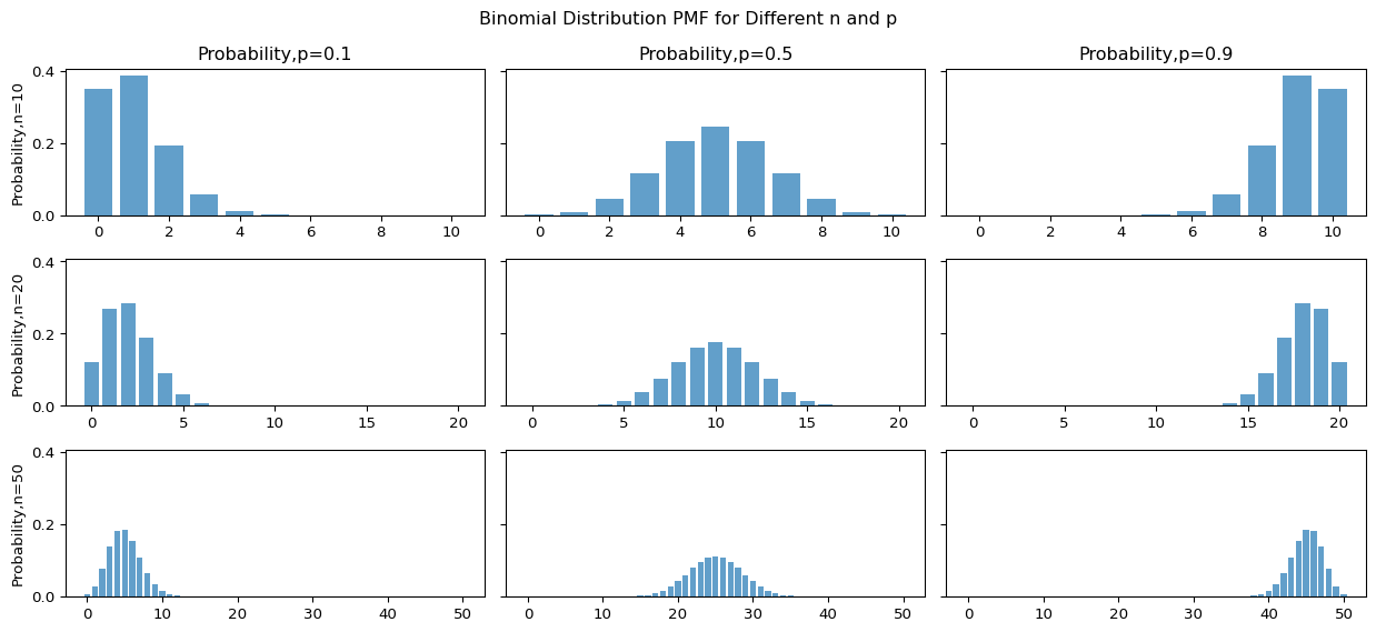
Binomial distribution
If a random variable \(X\) has a binomial distribution, we will write \(X \sim B(N,p)\).
Properties
- Support \(\mathcal{X} \in \{0, 1, \ldots, N\}\)
- Parameter \(N, p\), where
- \(p \in [0, 1]\) is the probability of success
- \(N\) is number of trials.
- pmf
\[ \small \begin{aligned} & P\left( X = x \mid N, p \right) = \binom{N}{x} p^x \, (1 - p)^{N - x} \end{aligned} \]
- Expectation: \(\mathbb{E}(X) = Np\)
- Variance: \(\mathbb{V}(X) = Np(1-p)\)
Analogy
We are tossing an unfair coins for 10 times with \(p(H) = 0.3\). What is the probability of
- getting 3 heads and 7 tails
- getting 7 heads and 3 tails
Illustration
Example: Wright-Fisher Model (Optional)
Consider a populaton with \(N\) diploid individuals. and we are interested in an allele with possibile genotypes \(A\) and \(a\)
- Each individual in the population produces a large number of gametes.
- Fixed population size
- Mendelian inheritance applied
Please describing the probability that there will be \(n_{A1}\) copies of \(A\) in the next generation given that there are \(n_{A0}\) copies in the parent generation:
\[ p(n_{A1} \text{in offspring}\mid n_{A0} \text{in parents})=\binom{2N}{n_{A1}}( \frac{n_{A0}}{2N} )^{n_{A1}}( 1-\frac{n_{A0}}{2N} )^{2N-n_{A1}} \]
Some Properties on Binomial distribution
- it is obvious us that p(x) for a binomial distribution is the (x+1)-th term in the expansion of \([p + (1-p)]^N\) (Binomial theorm)
- In this end, it is clear that binomial distribution satisfy the axiom
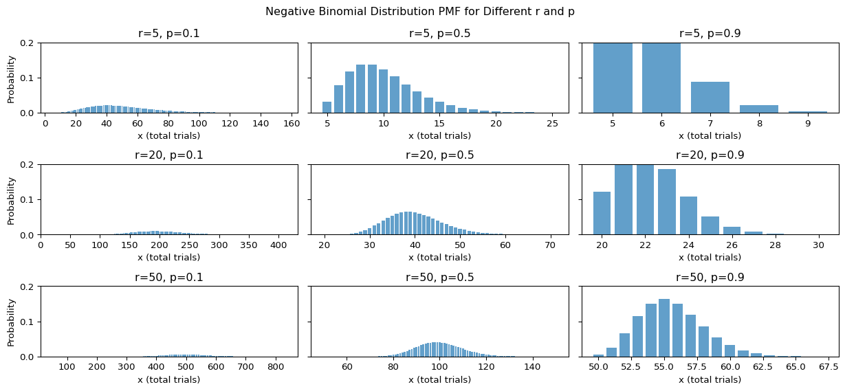
Negative binomial distribution
We define the random variable \(X\) as how many time we need to toss until the r-th success. \(X\) follows negative binomial distribution (\(X\sim NB(r,p)\))
Properties
- Support \(x\in\{ \mathbb{N} \mid\quad\forall \mathbb{N}>r\}\)
- Parameter \(r,p\)
- pmf
\[ P\left( X = x \mid r, p \right) \; = \; \binom{x - 1}{r - 1} p^r (1 - p)^{x - r} \]
- Mean \(\frac{r(1-p)}{p}\)
- Variance \(\frac{r(1-p)}{p^2}\)
Analogy
- Tossing coins to see how many times it take to see the 5-th head
- Gene expression
Illustration
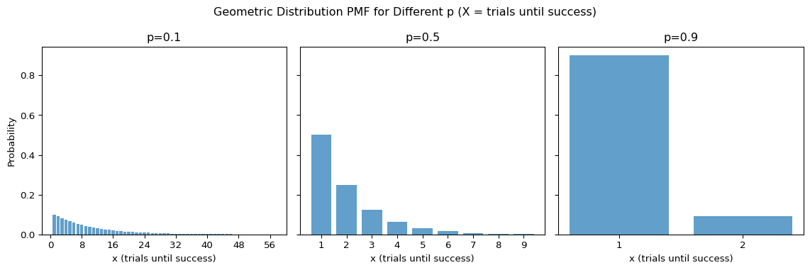
Geometric distribution
A geometric distribution special case of the negative binomial distribution where \(r = 1\).
A random variable \(X \sim G(p)\) follows geometric distribution has the following property
Properties
- Support \(x \in \mathbb{N}\)
- Parameter \(p\) is the probability of success
- pmf
\[ P\left( X = x \mid p \right) \; = \; p (1 - p)^{x - 1} \]
- Mean \(\frac{1}{p}\)
- Variance \(\frac{(1-p)}{p^2}\)
Analogy
A mobile game has a 5% draw a SSR card. In average, how many draws do you need to get a SSR card?
Illustration
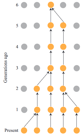
Example: Coalescent (Optional)
The probability that two alleles in generation \(t\) are copies of the same allele in generation \(t − 1\) is \(\frac{1}{2N_e}\) (i.e. probaility to coalesce).
For a coalescent event occur at \(t\) generation ago, it means that two alleles have NOT have colleased in the \(1 \dots t-1\) generation ago.
The probability that two alleles coalesced t generations ago
\[ P(T=t)=(1-\frac{1}{2N_e})^{t-1}(\frac{1}{2N_e}) \]
Hypergeometric distribution
Tthis time we draws sample without replacement from the finite sample \(N\) with known \(K\) succeess and the random variable \(X\) is defined as exactly \(x\) times of success with \(n\) draws. \(X\sim\text{Hypergeometric}(N,K,n)\)
Properties
- Support \(x \in {\max(0,n+K-N),\dots,\min(n,K)}\)
- Parameter \(N, K, n\)
- pmf
\(P( X = x) = \frac{\binom{K}{x}\binom{N-K}{n-x}}{\binom{N}{n}}\)
- Mean \(n\frac{K}{N}\)
- Variance \(n\frac{K}{N}\frac{N-K}{N}\frac{N-n}{N-1}\)
Analogy
Choosing 5 red balls and 3 blue balls from total 10 red balls and 15 blue balls without replacement
Example: Fisher’s exact test
We can view the p-value in Fisher’s exact test as the cdf of a hypergeometric disstribution.
| Tretment | Control | Row sum | |
|---|---|---|---|
| Y | a | b | M |
| Not Y | c | d | N-M |
| Column sum | n | N-n | N |
Fisher’s exact value assumes
the row sum&column sum value fixed
Observation of contingency table follows hypergeometric distribution with the probability:
\[ p(x=a) = \frac{\binom{M}{a}\binom{N-M}{n-a}}{\binom{N}{n}} \]
Example: Capture and Re-capture Experiment (Optional)
To estimate the population size of a specific animal in a certain region, the ecologists erform the following procedure (This methods were adopted in counting counting health survey, microbome)
- Catch \(m\) animal from the site, label them with marker and release.
- After a couple of time, catch \(n\) animal from the lake.
We denoted the number of marked animal as \(X\) and it is obvious that \(X\) follow hypergeometric distribution
In our experiment
- \(n\) animal caught
- \(i\) marked animal
so the probability of having \(i\) given the the unknown population parameter \(N\) is
\[ P(X=i | N)\frac{\binom{M}{i}\binom{N-M}{n-i}}{\binom{N}{n}} \]
Example: Capture and Re-capture Experiment (Optional)
- Finding optimal \(N\) is tough
- Trick: Consider
\[r=\frac{P(X=i | N)}{P(X=i | N-1)}\]
- \(P(X=i | N)\geq P(X=i | N-1)\) (i.e. \(r\geq 1\)) then we should use the parameter N as the estimation rather than \(N-1\)
- Optimal N will at the boundary condition
The boundary condition will be
\[ \begin{aligned} (N-m)(N-n) \geq & N(N-m-n+i) \\ \rightarrow & N \leq \frac{mn}{i} \end{aligned} \]
The best estimation of population size the larget integer less than \(\frac{mn}{i}\)